A compression perspective on curriculum learning

A fundamental property of an intelligent system is the ability to predict, be it predicting the label of an image, the optimal action to take, or the next token in a sentence. Having a good predictive model is intimately tied to having a good compression algorithm. Conversely, a strong compression algorithm must have a good model that can identify and leverage patterns in the data.

While the relationship between compression and intelligence has been thoroughly discussed¹, we will focus here on a particularly interesting relationship between compression and massively overparameterized models, which also naturally lends itself to an objective for data selection and curriculum learning.

Deep learning and the minimum description length (MDL) principle

Suppose Alice wants to send a dataset \(X = (x_1, x_2, \dots, x_n)\) to Bob over a noiseless communication channel that incurs some cost for each bit sent. We use \(L(\cdot)\) to denote description length, or the number of bits Alice needs to use in order to send an object to Bob. If \(X\) contains symbols (e.g., tokens or bytes) from a discrete vocabulary \(V\), then naively, each symbol can be encoded with \(\text{log} \thinspace |V|\) bits. So at first glance, the description length of the whole dataset is \(L(X)=n \thinspace \text{log} \thinspace|V|\) bits.

To minimize the number of bits sent, Alice can use a model \(M\) to compress \(X\). In particular, suppose \(M\) is a probabilistic model \(p_\theta(x_t \mid x_{<t})\) that predicts the next symbol based on the previous ones. By using an entropy coding (such as arithmetic coding), she can send \(x_t\) to Bob using \(-\log \thinspace p_\theta(x_t \mid x_{<t})\) bits. Then she can send the entire dataset using \(-\sum_{t=1}^n \text{log} \thinspace p_\theta(x_t \mid x_{<t})\) bits. If \(M\) is a good predictive model, then this could be much smaller than the naive cost of \(n \thinspace \text{log} \thinspace|V|\) bits.

However, this approach requires Bob to have the model \(M\), so that he can decode the data. Since Alice needs to send Bob the parameters \(\theta\) of this probabilistic model, the total description length of the dataset under this scheme is:

\[ L_M(X) = L(M) + L(X \mid M)=L(\theta) - \sum_{t=1}^n \text{log} \thinspace p_\theta(x_t \mid x_{<t}). \]

Graphically:

┌──────────────────────────────┐           ┌──────────────────────────────┐
│            Alice             │           │             Bob              │
└──────────────────────────────┘           └──────────────────────────────┘
         │                                              │
 train model M with weights θ                           │
         │                                              │
         │                                              │
         ├─────────────────── send θ ──────────────────►│
         │                                              │
         │                                          receive θ
         │                                              │
 encode x₁ using p_θ(x₁)                                │
   (emits message m₁)                                   │
         │                                              │
         ├───────── send m₁(-log p_θ(x₁) bits) ────────►│
         │                                              │
         │                                     decode m₁ with p_θ to get x₁
         │                                              │
 encode x₂ using p_θ(x₂)                                │
   (emits message m₂)                                   │
         │                                              │
         ├───────── send m₂ (-log p_θ(x₂) bits) ───────►│
         │                                              │
         │                                     decode m₂ with p_θ to get x₂
         │                                              │
         │                 ... repeat ...               │

The minimum description length principle (MDL, Rissanen, 1978; Grünwald, 2007) suggests the best model \(M\) for describing \(X\) is one that minimizes \(L_M(X)\). It has been influential as a guiding principle in machine learning, with applications ranging from model selection to regularization, model compression, and more (Barron & Cover, 1991; MacKay, 1992; Hansen & Yu, 2011).

The problem with applying the MDL principle to deep learning is that practical models are simply too “big.” If the model has billions of parameters, the upfront cost \(L(\theta)\) incurred when Alice sends \(\theta\) to Bob drowns out any gains from using the model to encode the dataset.

To make the problem worse, large models are often better than small models in practice, yet they often yield a larger description length \(L_M(X)\), due to the larger \(L(\theta)\). This leads to an apparent contradiction with the MDL principle where the model with larger description length is actually better. This problem comes from the fact that we don’t know how to compress large neural networks well, even though larger models have likely learned a simpler representation of the data².

Prequential coding

We now describe a different compression protocol for \(X\) called prequential coding³ that avoids many of the issues with the MDL protocol.

Since the main issue with the previous MDL approach is the cost \(L(\theta)\) of sending model parameters, the prequential coding approach avoids sending any model parameters. Instead, both Alice and Bob will separately train the same model as she sends him the dataset \(X\). In particular, the process looks as follows:

1. Alice sends Bob a deterministic training script \(\texttt{train.py}\) that initializes an LLM with a fixed random seed and implements its \(\texttt{update}\) function.
2. Alice and Bob both initialize their LLMs and obtain the same model \(p_{\theta_0}\) (since the random seed is fixed)
3. Alice encodes \(x_1\) with \(p_{\theta_{0}}(x_1)\) into a message \(m_1\) of length \(-\text{log} p_{\theta_{0}}(x_1)\), and sends the message to Bob
4. Bob receives \(m_1\) and uses \(p_{\theta_{0}}\) to decode \(x_1\).
5. Now both Alice and Bob have \(x_1\) and they both take a gradient step on \(x_1\) according to \(\texttt{train.py}\), \(\theta_1 = \texttt{update}(x_0, \theta_0)\) and end up with the same copy of \(\theta_1\).
6. Go to step 3 and repeat until the whole dataset has been sent.

Graphically:

┌──────────────────────────────┐           ┌──────────────────────────────┐
│            Alice             │           │             Bob              │
└──────────────────────────────┘           └──────────────────────────────┘
         │                                              │
         |                                              │
         ├──────── (1) send train.py and seed ─────────►│
         │                                              │
  (2) initialize θ₀                           (2) initialize θ₀
         │                                              │
  (3) encode x₁ using p_θ₀(x₁)                          │
      (emits message m₁)                                │
         │                                              │
         │                                              │
         ├──────── send m₁ (-log p_θ₀(x₁) bits) ───────►│
         │                                              │
         │                               (4) decode m₁ to recover x₁
         │                                              │
(5) update θ₁ = update(θ₀, x₁)          (5) update θ₁ = update(θ₀, x₁)
         │                                              │
         ├──────────────────────────────────────────────│
         ├──────────────────────────────────────────────│
         │                                              │
  (3) encode x₂ using p_θ₁(x₂)                          │
       (emits message m₂)                               │
         │                                              │
         │                                              │
         ├──────── send m₂ (-log p_θ₁(x₂) bits) ───────►│
         │                                              │
         │                               (4) decode m₂ to recover x₂
         │                                              │
  (5) update θ₂ = update(θ₁, x₂)        (5) update θ₂ = update(θ₁, x₂)
         │                                              │
         │                  ... repeat ...              │

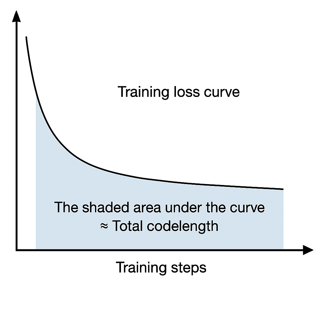
Under this setup, the total number of bits Alice needs to send to Bob in order to communicate \(X\) is:

\[L_\text{PC}(X) = L(\texttt{train.py}) + \sum_{t=1}^n L(m_t) = L(\texttt{train.py}) -\sum_{t=1}^n \text{log} \thinspace p_{\theta_t}(x_t \mid x_{<t}). \]

Notice that the second term is adding up the loss of the model at each training step \(t\), so it is precisely the area under the training loss curve (AULC).

The first term \(L(\texttt{train.py})\) can be negligible compared to the size of \(X\): a minimal implementation for training a neural network is quite small⁴, and it does not grow with model or dataset size. Unlike in the MDL picture, Alice never has to send Bob the model parameters so increasing model size does not increase the description length. In fact, larger models result in better compression under prequential coding since larger models tend to train faster, so this coding scheme is particularly suitable for deep learning (Blier & Ollivier (2018)).

This algorithm can achieve a great compression ratio but it is not very practical since both the compression and decompression processes require training a model. In fact, one of the most powerful instantiations of prequential coding is the Solomonoff Induction, a mathematically optimal but unfortunately incomputable procedure for sequence induction.

Connection to data selection and curriculum learning

Previously, we assumed Alice sends the dataset \(X\) to Bob in some order \(x_1, x_2, x_3, \cdots\). But the ordering of messages is actually a choice because the dataset \(X\) is typically made up of exchangeable documents⁵, which we denote by \(d_i\):

\[ X = (\underbrace{x_1, x_2, x_3}_{d_1}, \underbrace{x_4, x_5, x_6, x_7}_{d_2}, \dots) = (\underbrace{x_4, x_5, x_6, x_7}_{d_2}, \underbrace{x_1, x_2, x_3}_{d_1}, \dots). \]

Since Alice can send documents to Bob in any order she wants, she can choose an ordering that minimizes the description length. If some documents contain information that is shared across many documents, sending them first could help reduce the number of bits required to send later documents.

As we saw earlier, this is equivalent to choosing the ordering of documents that minimizes the AULC, so we arrive at a neat and principled objective for curriculum learning and data selection. This objective is also intuitive from a learning perspective: training on certain documents first could make it easier to learn other documents later on, leading to a lower AULC.

Formally, suppose we have \(n_D\) documents, and we are training a model with stochastic gradient descent for a single epoch (the model sees every symbol once). Our objective is to find a curriculum, or an ordering of the \(n_D\) documents that minimizes the description length. In our setting, this is equivalent to finding a permutation \(\sigma:[n_D] \rightarrow [n_D]\) of the documents (i.e., a bijection between orderings) that minimizes the area under the training loss curve⁶:

\[ \text{arg}\min_\sigma -\sum_{t=1}^{n_D} \text{log} p_{\theta_t}\left(d_{\sigma(t)} \mid d_{\sigma(1)}, \cdots, d_{\sigma(t-1)}\right). \]

Solving this problem is computationally challenging in practice because the number of permutations is factorially large. If computation resource is not a constraint, a straightforward strategy would be to train every permutation and pick the one with the smallest AULC. This strategy is not practical, but it would be nonetheless useful to know whether there exist permutations that are better than random. In Adaptive Data Optimization (ADO), we demonstrate a meta-learning approach that can find good permutations for training small multi-layer perceptrons (MLPs). Our meta-learning method produces a curriculum that significantly outperforms training on randomly shuffled documents. This result shows it is likely that good curricula exist for most realistic problems, but they are computationally difficult to find. We refer the interested reader to Appendix B of the ADO paper for details.

Although our example here focuses on single-epoch training with minibatch size 1, the prequential coding perspective on data selection is much more general. For example, Alice and Bob are not obligated to train the model on individual data points as they are being transmitted. They can choose to skip updating the model on some data points or choose to train more on data that has already been transmitted (similar to experience replay). Additionally, Alice can choose to skip sending some data points and transmit all of the skipped data points at the end without updating the model–this is equivalent to data filtering⁷.

A practical approach

The meta-learning approach above works for small neural networks, but does not scale to practical settings. To design a practical method for data selection, we need to make some assumptions about the problem’s structure.

One popular structural assumption is that documents can be grouped into different domains. For example, we could group all documents from Wikipedia into one domain and all documents from Reddit into another domain. Under this grouping strategy, a well known dataset such as The Pile has 22 domains. We assume that documents within each domain are approximately homogeneous, so that training on one document gives “similar” information as training on other documents. This drastically simplifies the data selection problem, since we only need to find a curriculum over the domains instead of over all documents. In particular, at each training step \(t\) we can output a mixture distribution \(\pi(t) \in \Delta^K\) controlling how we sample mini-batches from \(K\) domains. Still, even with the imposed structure of domains, the optimization remains difficult.

The hardest part of optimizing data mixtures is that it is hard to know the performance of a model on a data mixture without actually training on it, but training a model to test each proposed data mixture is expensive. ADO resolves this issue by fitting per-domain scaling laws that model the loss curve on each domain as a function of the number of total data points seen. Scaling laws are very cheap to fit, and can reliably forecast the loss of domains into the future. This allows us to continuously estimate the per-domain loss curves throughout the training, and adjust the data mixture in response. ADO is designed as a method that greedily tunes the mixture to optimize the loss AULC, using the loss curve forecasts provided by scaling laws. Under the prequential coding framework, we can view this as greedily minimizing the total number of bits required to communicate the training dataset.

ADO is a practical method because it adds minimal computational overhead and achieves better downstream performance than competing methods. That being said, ADO actually does not minimize the observed AULC in practice, but that is a topic for a different blog post on algorithmic information theory :)

Final thoughts

We introduce a natural, principled objective for curriculum learning and data selection via prequential coding, by casting curriculum design as explicit minimization of the training‐loss AULC. While naively optimizing this objective is intractable, we believe that this compression‐driven viewpoint could be an elegant and promising principle on which new data selection and curriculum learning algorithms can be designed. For a more detailed discussion on Adaptive Data Optimization (ADO), see this blog post.